Plot silhouette scores from clustering results
Source:R/plot_ulrb_silhouette.R
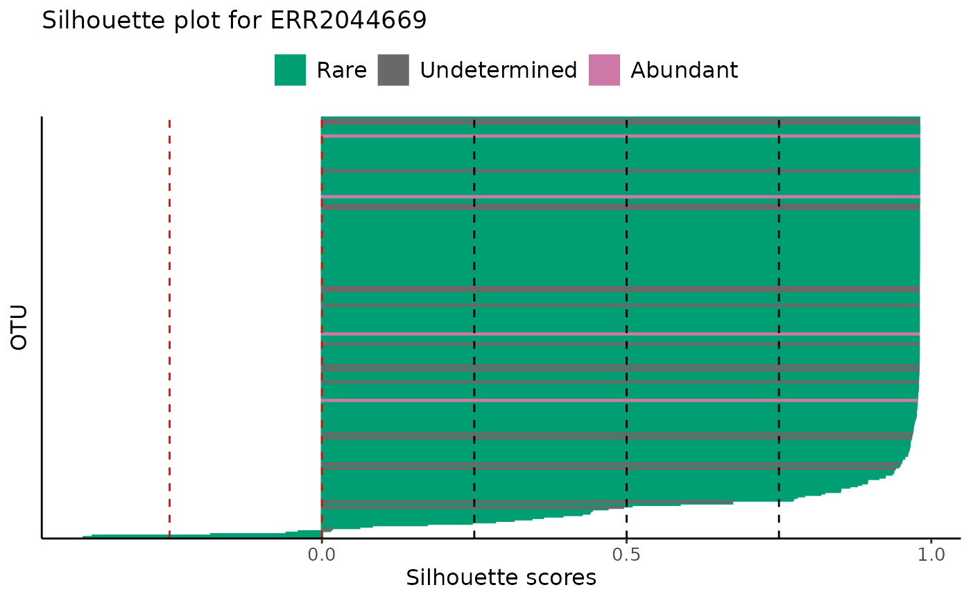
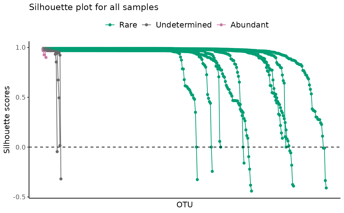
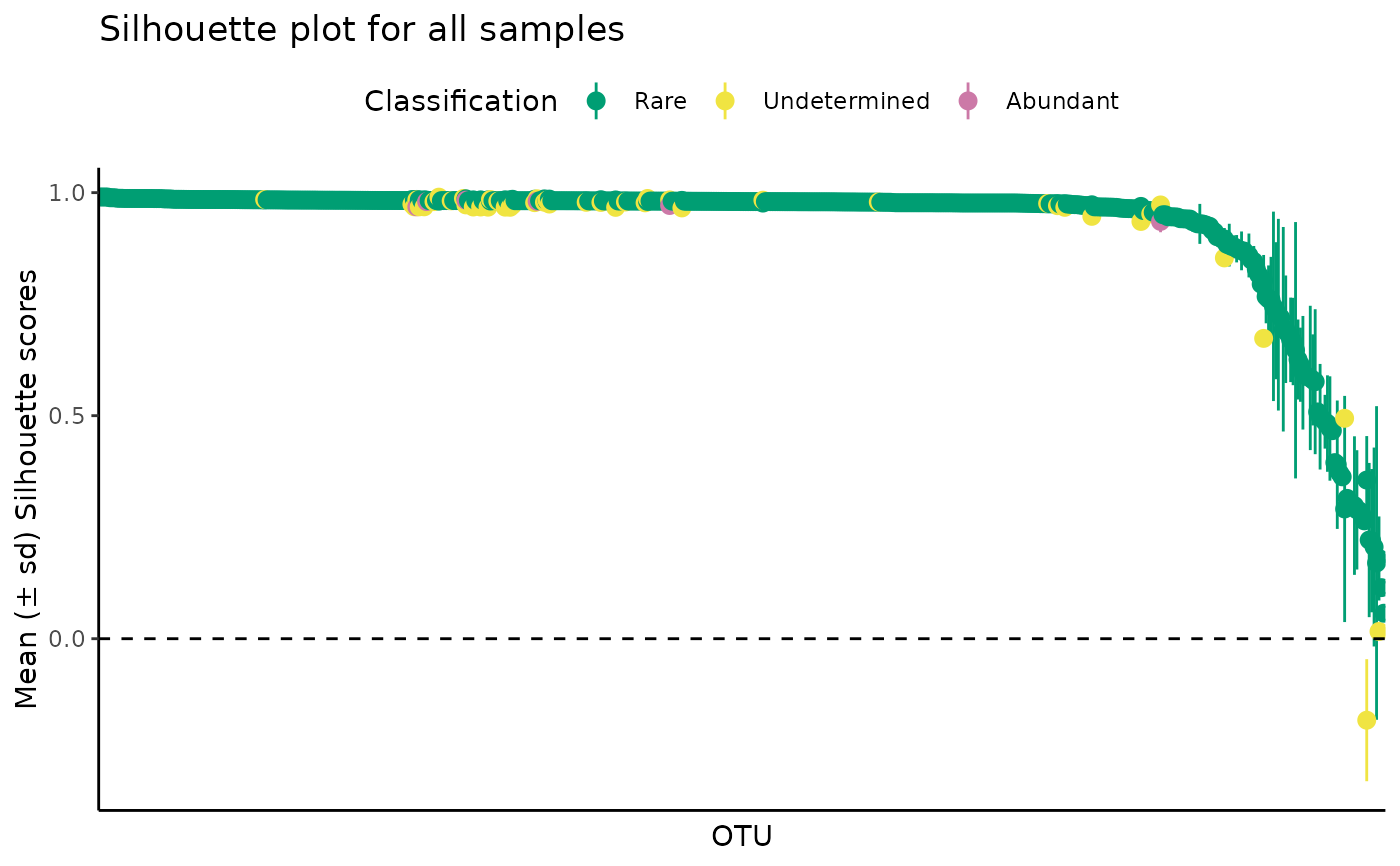
plot_ulrb_silhouette.RdPlots the Silhouette scores from the clustering results of define_rb().
Usage
plot_ulrb_silhouette(
  data,
  sample_id = NULL,
  taxa_col,
  samples_col = "Sample",
  plot_all = TRUE,
  classification_col = "Classification",
  silhouette_score = "Silhouette_scores",
  colors = c("#009E73", "grey41", "#CC79A7"),
  log_scaled = FALSE,
  ...
)
Arguments
- data
...
- sample_id
string with name of selected sample.
- taxa_col
string with name of column with phylogenetic units. Usually OTU or ASV.
- samples_col
name of column with sample ID's.
- plot_all
If TRUE, will make a plot for all samples with mean and standard deviation. If FALSE (default), then the plot will illustrate a single sample, that you have to specifiy in sample_id argument.
- classification_col
string with name of column with classification for each row. Default value is "Classification".
- silhouette_score
string with column name with silhouette score values. Default is "Silhouette_scores"
- colors
vector with colors. Should have the same lenght as the number of classifications.
- log_scaled
if TRUE then abundance scores will be shown in Log10 scale. Default to FALSE.
- ...
other arguments.
Details
This works as a sanity check of the results obtained by the unsupervised learning method used to classify taxa. This is specially important if you used an automatic number of clusters.
The function works for either a single sample (that you specify with sample_id argument), or it can apply a centrality metric for taxa across all your samples (plot_all = TRUE).
For more details on Silhouette score, see check_avgSil() and cluster::silhouette().
Interpretation of Silhouette plot
Based on chapter 2 of "Finding Groups in Data: An Introduction to Cluster Analysis." (Kaufman and Rousseeuw, 1991); a possible interpretation of the clustering structure based on the Silhouette plot is:
0.71-1.00 (A strong structure has been found);
0.51-0.70 (A reasonable structure has been found);
0.26-0.50 (The structure is weak and could be artificial);
< 0.26 (No structure has been found).
Examples
classified_species <- define_rb(nice_tidy)
#> Joining with `by = join_by(Sample, Level)`

# Standard plot for a single sample
plot_ulrb_silhouette(classified_species,
                       sample_id = "ERR2044669",
                       taxa_col = "OTU",
                       abundance_col = "Abundance",
                       plot_all = FALSE)

# All samples in a dataset
plot_ulrb_silhouette(classified_species,
          taxa_col = "OTU",
          abundance_col = "Abundance",
          plot_all = TRUE)


# All samples with a log scale
plot_ulrb_silhouette(classified_species,
          taxa_col = "OTU",
          abundance_col = "Abundance",
          plot_all = TRUE,
          log_scaled = TRUE)
